
Overview
Deep learning with Deep Neural Network has gained huge momentum in the past few years owning to the blooming of data and GPU accelerated computation. The former makes it possible to collect massive amount of training data to tune millions or even billions of parameters; the later makes running deep learning computation approachable for everyone have access to a consumer PC with GPU installed.
One of the most exciting fields of deep learning application is computer vision which gives machine the ability to see. One of the most influential innovations in the field of computer vision is Convolutional Neural Network(CNN), first published by LeCun et al [1], became prominence as Alex Krizhevsky used it to win 2012 ImageNet competition.
Though empowered by GPU, building an image classifier with CNN still takes a long time to train. Besides CNN needs to go deeper to achieve good result on more complex tasks which requires massive amount of training data for tuning the weights.
If we imagine how we learn as a human, we do not learn to recognize every object from stretch. After learning how a bike looks like and how it works, even for the first time we see a car, we can immediate transfer our knowledge from bikes and give a fairly close prediction to how a car may be used.
Similarly after training a network to learn dogs and cats, we should not have to learn to classify a wolf and tiger from stretch because we have already learned how the face and body look like for dog or cat like animals.
There are many sophisticated CNN models already pretrained with ImageNet images. i.e. it has learned to classify the 1000 objects in the ImageNet and have also learned the parts that assembles them. We then just have to transfer the knowledge to our tasks without having to learn the basic elements of objects from stretch. This will solve our problem as it greatly reduces the number of trainable weights in our model which requires way less data and effort to learn.
In this blog, I will train an image classifier using the KTH-ANIMALS dataset[3] to classify 19 different animals with CNN.
Jupyter notebook for this blog is available here.
Data Exploration
The KTH-ANIMALS dataset[3] contains only 1740 images in total and are of different shapes from ~200 to ~400 pixels width and height. Figure 1 shows the images in their original shape.
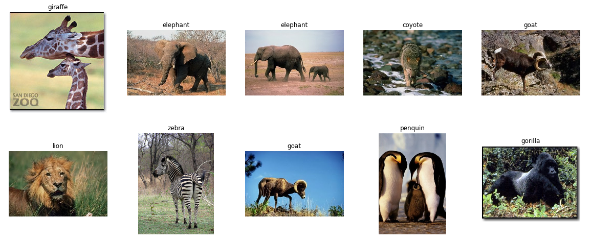 Figure 1: Images as original shape
Exploratory Visualization
KDE plot of R,G,B channels for each class tells us the color distribution for each class. Animals in dark yellow such as coyote, horse, leopard, lion and tiger contributes to the peaks on the left of the red channel. These pictures are taken in the wild which explains the significant amount of dark green and dark blue in most classes due to the grass field and the sky.
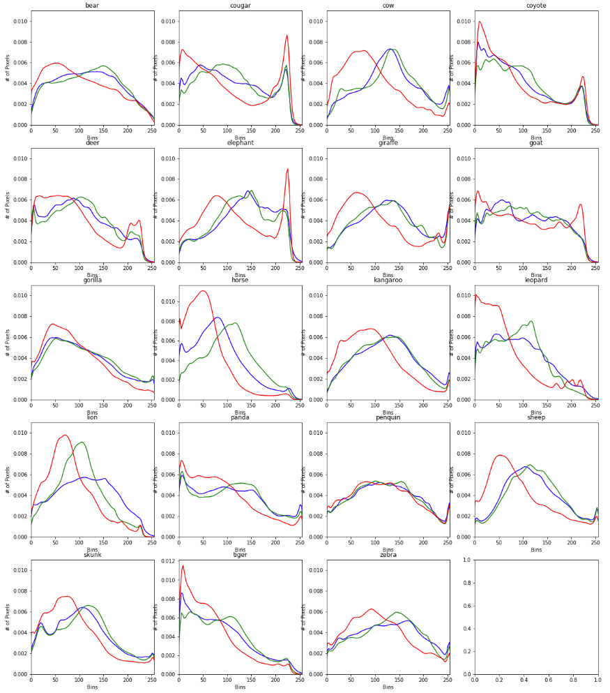 Figure 2: KDE plot by class
Training data count by class shows the dataset is quite evenly distributed.
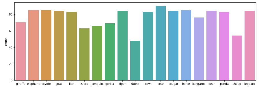 Figure 3: Image count by class
Data Preprocessing
I randomly splitting the data into training, validation and test set containing 1460, 180 and 100 images respectively. Leaving us merely 78 images on average per class which is far from sufficient to train a CNN model from stretch to classify such a diverse dataset. Add another 40 images from Google to the test set (140 images in total).
Images are loaded as 224x224 pixels images. Figure 4 shows the images loaded.
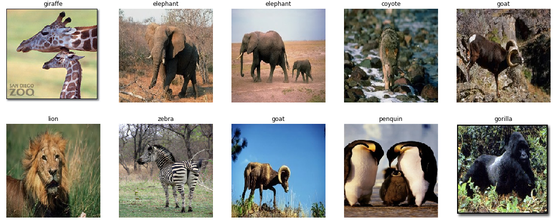
Figure 4: Images loaded as 224x224
Image Augmentation is applied to training data to combat overfitting and to make the models more robust.
datagen = ImageDataGenerator(
    rotation_range=10,
    shear_range=0.2,
    zoom_range=0.2,
    horizontal_flip=True,
)
Figure 5 shows the augmented images.
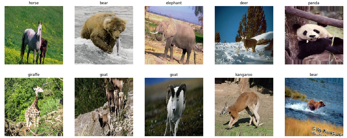
Figure 5: Images Augmented
Benchmark Model
Our benchmark model - a CNN model contains 5 Convolutional layers - similar architecture to VGG19 except that every block has only one CNN layer and Global Average Pooling(GAP) is used instead of Fully Connected(FC) layer to reduce overfitting.
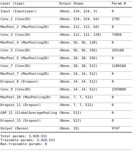
Figure 6: Benchmark Model
A simpler model tend to easily overfit(or underfit if too simple) while a deeper model cannot learn due to the limitation of the insufficient number of training data.
It took 259.6 seconds, 29 epochs to finish training the benchmark model. 8.95 seconds per epoch. On test dataset, it achieves 57% accuracy, 0.5479 kappa score and 1.83 cross-entropy loss at the 23th epoch.
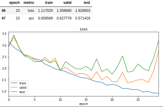
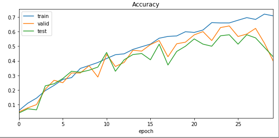
Figure 7: Benchmark Model Result
Transfer Learning
I first build a transfer learning model - a VGG19 with weights pre-trained on ImageNet dataset with top layers(two FC layers) replaced with a top model.
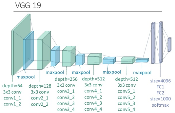
Figure 8: VGG19
Figure 9 shows the Top Model used to replace the two FC layers and the output layer (in purple above).
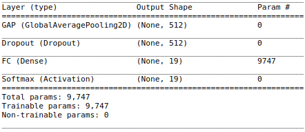
Figure 9: Top Model
To train the Top Model , we need to pass the training, validation and test dataset through the VGG19 (without top layers included) to obtain the input features (bottleneck features) for the top model.
# Load pre-trained VGG19
pretrained_model = applications.VGG19(include_top=False, weights='imagenet')

# Generator for augmented training data
train_X_generator = datagen.flow(X_train, batch_size=batch_size, shuffle=False)

# Generate bottleneck features
bottleneck_features_train = pretrained_model.predict_generator(train_X_generator, steps=len(X_train) / batch_size)
bottleneck_features_valid = pretrained_model.predict(X_valid)
bottleneck_features_test = pretrained_model.predict(X_test)
I then use the bottleneck features as the input to train the weight of the top model.
It took 40.83 seconds, 235 epochs to finish training the top model. Merely 0.17 second per epoch. Achieve 60% test accuracy, 0.5777 kappa score and 1.41 log loss at the 224th epoch.
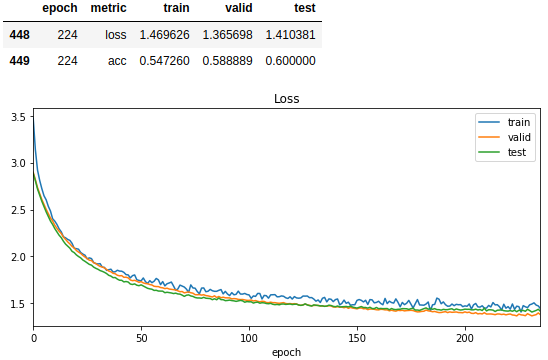
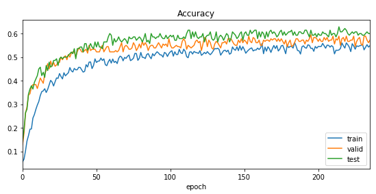 Figure 10: Top Model Result
Fine-Tune Transfer Model
I connect the Top Model trained above to the pretrained VGG19(with top layers removed) to build a new model. This new model at this point is exactly the same as the Top Model above if feeding the 4D tensor rather than the bottleneck features as inputs.
I then freeze the first 4 CNN blocks of VGG19 to fine tune the last (5th) block of VGG19 as well as our Top Model. By freezing the first 4 CNN blocks, we can freeze the pre-trained weights applicable to general image classification task. Fine tuning the more abstract layers so that the last CNN block learns the high level features related to this task.
model = Sequential()

# Add VGG19 (without top layers)
for l in pretrained_model.layers:
    model.add(l)

# Add my Top Model
for l in top_model.layers:
    model.add(l)

## Lock layers until the last ConvNet block
lock_until = 17
for n, layer in enumerate(model.layers):
    if n < lock_until:
        layer.trainable = False
    else:
        layer.trainable = True
Here is the model with weights trainable from block5conv1.
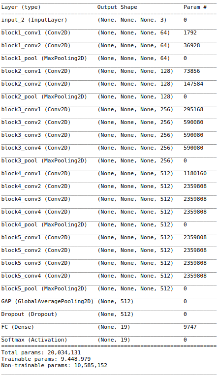 _Figure 11: Fine-Tuned Model
It took 375.82 seconds, 30 epochs to finish fine tuning the model. 12.5 seconds per epoch. Achieve 80% test accuracy, 0.7890 kappa score and 0.93 log loss at the 24th epoch. Another +20% improvement in test accuracy.
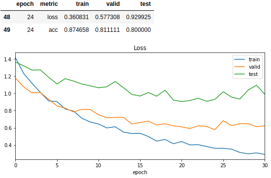
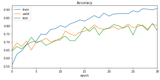 Figure 12: Fine-Tuned Model Result
Result
As shown in Table 1, the power of transfer learning is already showing in the top model. Training the top model is 53x faster while achieving a better result. The fine-tune model significantly improve the model in all metrics.
| Metrics on Test Dataset | Training Time/Epoch | Cross-Entropy Lost | Accuracy | Kappa Score |
|---|---|---|---|---|
| Benchmark Model | 8.95s | 1.83 | 57% | 0.5479 |
| Top Model | 0.17s | 1.41 | 60% | 0.5777 |
| Find-Tuned Model | 12.5s | 0.93 | 80% | 0.7890 |
Table 1 Model Evaluation
Conclusion
This blog post demonstrated how powerful transfer learning is by outperforming a non-trivial CNN model trained from stretch with just a fraction of the training time which insufficient training data. Also how pretrained model can be further fine-tuned to obtain massive performance improvement that could not otherwise be achievable if training a new CNN model. We can see huge potentials applying transfer learning in real life applications especially in testing out new ideas quickly without having to collect a huge amount of train data and a long training time.
Reference
[1] http://yann.lecun.com/exdb/publis/pdf/lecun-99.pdf
[2] https://www.cs.princeton.edu/~rajeshr/papers/icml09-ConvolutionalDeepBeliefNetworks.pdf
[3] https://www.csc.kth.se/~heydarma/Datasets.html
[4] https://arxiv.org/pdf/1311.2901.pdf
[5] https://blog.keras.io/building-powerful-image-classification-models-using-very-little-data.html
[6] https://www.kaggle.com/wiki/LogLoss
[7] http://cnnlocalization.csail.mit.edu/Zhou_Learning_Deep_Features_CVPR_2016_paper.pdf
[8] https://alexisbcook.github.io/2017/global-average-pooling-layers-for-object-localization/