Overview

Deep learning model is often a black box. It’s usually hard to understand how the deep neural network learned the features based on which it makes predictions. This blog post will show a technique introduced by Zhou et al[1] that could help us understand what the CNN has learned from the training and based on what it makes predictions.

Code is available here (at the bottom).

The CNN Model

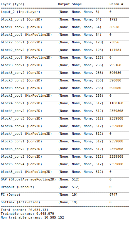
The model use here is the VGG19 I built in this post with the last two FC layers (before the output layer) replaced with a GAP (Global Average Pooling) layer.

The model is used to classify 19 different animals.

How it works

I use GAP instead of FC(Fully Connected) layers not only to reducing overfitting but also it brings an interesting byproduct - weights of the last CNN can be used for nearly effortless object localization which also serves as a window to peak inside a CNN how it makes predictions.

The idea behind is simple. When using GAP layer before the final FC layer. The weights (512x1 vector - blue dotted lines in Figure 1) connecting GAP to each of the output node, e.g. panda, tell us which of those 512 feature maps activate the output. And each of the 512 nodes in GAP layer is calculated by averaging a 7x7 feature map, green dotted lines below.

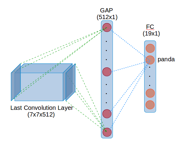
Figure 1: Weights to Activation Map

Therefore multiplying 7x7x512 by 512x1 gives us the weighted feature map - the activation map which allow us to visualize which part of the image is activating that particular output class. Below I will show it in action.

A New Model

We need to create a new model - from the existing CNN model and use the last CNN layer weights as a secondary output.

• Build a new model
  First we need to add an extra output from the last Convolutional Layer.

  last_cnn_layer = -6  # the last convolution layer
  output_layer = -2    # the last layer (-1) is softmax activation in the current setting
  new_model = Model(inputs=model.input, outputs=(model.layers[last_cnn_layer].get_output_at(1), model.layers[output_layer].get_output_at(1))) 
  

• Get convolution output and prediction
  Pass the image through the model to obtain the last convolution output as well as the predicted class

  # get filtered images from convolutional output + model prediction vector
  last_conv_output, pred_vec = new_model.predict(img_path_to_tensor(img_path))
  last_conv_output = np.squeeze(last_conv_output)  # (1, 14, 14, 512) --> (14, 14, 512)
  pred = np.argmax(pred_vec) # get predicted class
  

• Get the FC layer weight (512x1)
  Get the FC layer weight that conneted to the predicted class. Multiply the last convolution output (14x14x512 - green dotted lines) by the FC layer weight (512x1 - blue dotted lines)

  all_fc_layer_weights = model.layers[output_layer].get_weights()[0]  # 512x19 (19 classes)
  fc_layer_weights = all_fc_layer_weights[:, pred] * -1 # 512x1
  activation_map = np.dot(last_conv_output, fc_layer_weights) # 14x14x512 * 512x1 = 14x14 
  

Activation Map

Passing below image with two pandas through the steps above returns a 14x14 activation map using the weights of the predicted animal ‘panda’. 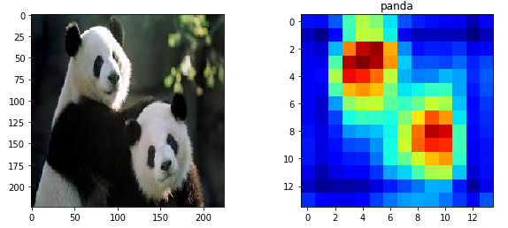Figure 2: Activation Map

Upsampling the activation map 16 times (224x224) and overlay it on top of the original image shows that the model predicts panda mostly due to the iconic look of its face.

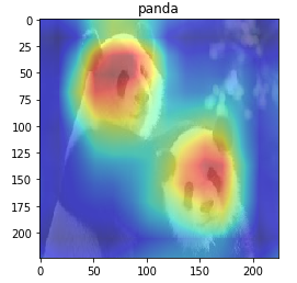Figure 3: Activation Map Overlay

The activation map is also used as object localization.

How CNN Make Predictions

To peak into the CNN black box. I randomly picked 15 classes and downloaded 1 picture for each class. Figure 4 shows that the model correctly classified all new images and also showing what the CNN is looking at when predicting the class label. For example, The elephant’s body and nose; The patten on the body of zebras and leopards; The black and white pattern of pandas, etc. These are strong evidences the CNN model has learned to identify animals by their key difference from the others.

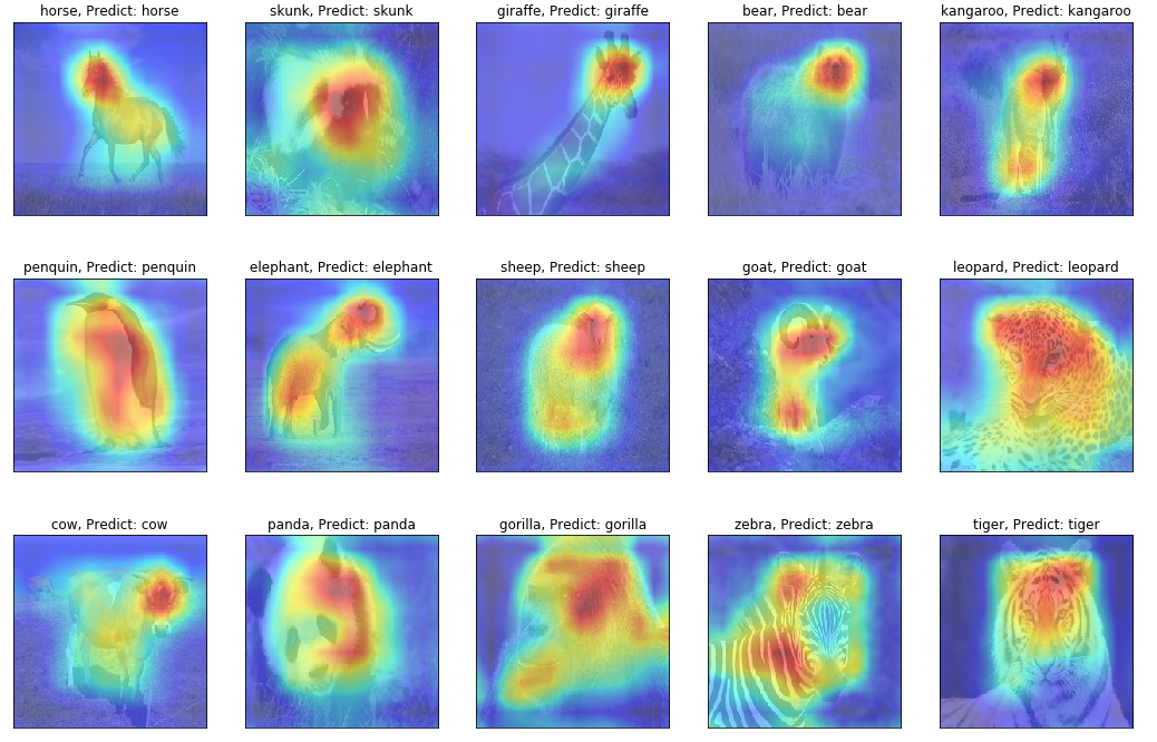Figure 4: CNN object localization

Going Further

We have demonstrated an interesting byproduct of CNN model using GAP layer. Potentially when dealing with images with multiple objects, we could use some of the highest scored (not just the best) FC weights to build the activation map to obtain the location of objects recognized by the mode then further feed the sub-images containing the objects through the CNN again to obtain the classes for all bounding boxes. Other studies have been made to utilize this method for more robust object localization, such as the study by Singh and Lee [3] where they expand the bounding box by randomly turning off parts of the training images to force the network to learn other parts of the object (not just the most iconic parts).

Reference

[1] http://cnnlocalization.csail.mit.edu/Zhou_Learning_Deep_Features_CVPR_2016_paper.pdf
[2] https://alexisbcook.github.io/2017/global-average-pooling-layers-for-object-localization/
[3] http://krsingh.cs.ucdavis.edu/krishna_files/papers/hide_and_seek/my_files/iccv2017.pdf